Propagation delay is a fundamental concept in PCB design, affecting whether high-speed circuits operate reliably or fail unexpectedly. As signal speeds increase in modern electronics, even tiny timing mismatches—ranging from a few to several tens of picoseconds—can lead to data errors, timing violations, or degraded signal quality. High-speed digital systems such as DDR memory interfaces, PCIe links, USB4, and multi-Gbps SerDes are particularly sensitive to these effects.
In diesem Artikel, PCBCool will explore PCB propagation delay through five main sections, covering definitions, causes, significance, calculations, and practical management techniques.
Propagation delay (often written as t_pd or tpd) is the time needed for an electrical signal to travel from its source, such as a driver pin, to its receiver, such as a load pin, along a PCB trace that acts as a transmission line.
In ideal wires, signals seem to arrive instantly. In real PCB traces, however, signals move at a limited speed. They typically travel at 60–70% of the speed of light in a vacuum (c ≈ 3 × 10^8 m/s, or roughly 11.8 inches per nanosecond). This delay occurs because the electromagnetic fields around the conductor interact with the dielectric material of the PCB, which slows the signal.
The propagation delay per unit length can be calculated as the inverse of the signal velocity:
t_pd = 1 / v
where v is the velocity of the signal in the medium. In vacuum or air, t_pd is about 85 picoseconds per inch. On PCB, this value increases due to the dielectric constant (Dk or ε_r) of the substrate. For standard FR-4 material (Dk ≈ 4.0–4.6), typical values are:
- Mikrostrip (trace on an outer layer with one side exposed to air): 145–150 ps/in
- Stripline (trace fully embedded between two reference planes): 170–171 ps/in
Microstrip traces are slightly faster because part of the electromagnetic field travels through air (Dk = 1). Stripline traces are slower but provide better shielding and more uniform signal conditions.
A useful rule of thumb is that signals travel about 6 inches per nanosecond on typical FR-4 boards. For example, a 6-inch trace introduces roughly 1 ns of delay, which becomes significant when rise times fall to a few hundred picoseconds in high-speed circuits.
Propagation delay is different from gate delay (the switching time inside an integrated circuit) or transmission delay (the time to send a full packet or bit stream). It refers only to the physical travel time along the interconnect, making it a crucial concept for understanding PCB signal timing.
Multiple factors control propagation delay, with the most important being the effective dielectric constant (ε_eff or Dk_eff).
The propagation delay per unit length can be estimated using:
t_pd ≈ 85 × sqrt(ε_eff) (for typical FR-4 PCB materials)
Or more generally:
t_pd = (sqrt(ε_eff) × L) / c
where L is the trace length and c is the speed of light in vacuum (with consistent units).
For microstrip traces, ε_eff is lower than the bulk Dk because some of the electromagnetic field extends into air.
For stripline traces, ε_eff is nearly the same as the bulk Dk since the field is fully confined in the dielectric.
Other important factors include:
- Dielectric constant of the material: Standard FR-4 has Dk ≈ 4.2–4.6, giving t_pd ≈ 174 ps/in for embedded traces. Low-Dk materials like Rogers RO3003 (Dk ≈ 3.0) or Isola Astra MT77 reduce this to around 136 ps/in for microstrip.
- Trace type and geometry: Microstrip is faster due to air exposure, while stripline is slower but more consistent.
- Trace length: Delay increases proportionally with length.
- Dielectric thickness and reference plane distance: These affect the field distribution and ε_eff.
- Other effects: Solder mask adds a thin layer with its own Dk; temperature and humidity can shift Dk by 5–10% in FR-4; copper surface roughness slightly affects signals above 10 GHz; via stubs add localized delay.
Variations in Dk across layers or board regions can lead to differences in signal velocity, causing timing skew—differences in signal arrival times across multiple traces. In modern designs with dense layouts and edge rates below 50 ps, tight stackup control is essential to manage these effects.
In low-speed circuits, propagation delay is negligible compared to logic gate delays. As operating frequencies rise and signal edges become sharper, however, propagation delay becomes critical.
A trace should be treated as a transmission line when its round-trip delay approaches or exceeds the signal rise or fall time. Formally, the critical trace length can be estimated as:
L_critical ≈ t_r / (2 × t_pd)
If this condition is met, unmanaged traces can exhibit reflections, ringing, and impedance mismatches.
Specific problems caused by propagation delay include:
- High-speed serial links (PCIe Gen5/Gen6 at 32–64 GT/s, USB4, 100+ Gbps Ethernet): Small skew levels reduce eye opening, increase bit error rates, and add jitter.
- Parallel interfaces (DDR4/DDR5 memory): Data, address, command, and strobe signals must arrive within very narrow windows (often <50 ps for DDR5); differences lead to setup or hold failures.
- Differential pairs: Skew within a pair (positive vs. negative) creates common-mode noise, affecting EMI performance and noise rejection. Skew between pairs disrupts bus timing.
- Clock distribution: Differences between clock paths can cause synchronization problems across components.
A practical example: for a 100-ps rise time on FR-4 microstrip (150 ps/in), the critical trace length is only ~0.33 inches. Such short traces demonstrate how even small propagation delays become significant at high speeds.
In modern designs with sub-100-ps edges, high-density interconnects, and compact packaging, unmanaged delay can cause unreliable prototypes, compliance test failures, and field issues. Careful delay control is essential to build stable multi-Gbps systems, reduce errors, minimize skew, and improve signal integrity.
The total propagation delay of a PCB trace can be estimated as:
Total delay = t_pd × Trace length
where t_pd is in ps/in and length is in inches.
Simple estimate:
- For FR-4 microstrip, t_pd ≈ 150 ps/in.
- Delay in nanoseconds ≈ length / 6.67.
More accurate formulas:
t_pd ≈ 85 × sqrt(ε_eff) (microstrip)
t_pd ≈ 85 × sqrt(ε_r) (stripline)
To determine the maximum trace length for a target delay:
length = Desired delay / t_pd
Example 1: DDR interface with skew tolerance < 20 ps on FR-4 microstrip:
Max length mismatch = 20 ps / 150 ps/in ≈ 0.133 in ≈ 3.4 mm
Tools for higher accuracy:
- Pre-layout field solvers (Altium, Cadence Allegro, HyperLynx) to calculate ε_eff based on stackup and trace geometry.
- SPICE or IBIS simulation to predict full path delays, including vias.
- Measurement using Time-Domain Reflectometry (TDR) to capture round-trip delay (divide by 2), or Vector Network Analyzers (VNA) for phase delay in the frequency domain.
Practical example:
A 12-inch FR-4 microstrip trace has total delay ≈ 1.8 ns (150 ps/in).
With a 200-ps rise time, the trace behaves as a transmission line and requires controlled impedance and termination to prevent reflections.
Reverse example:
For a PCIe intra-pair skew requirement < 50 ps, lengths must match within 50 / 150 ≈ 0.33 in (≈8.4 mm).
These calculations and measurements help set trace routing guidelines in electronic design automation (EDA) tools.
To manage propagation delay and reduce skew, designers can follow several approaches:
Material Selection
- Use low-Dk and low-loss laminates such as Megtron 6, Rogers 4350B, or Isola Tachyon to lower baseline delay and reduce signal dispersion.
- Especially important for high-speed (>10 Gbps) or high-frequency designs.
Length Matching and Tuning
- Match electrical lengths rather than just physical lengths, accounting for ε_eff differences.
- Add serpentine (meander or accordion) patterns to shorter traces.
- Place tuning sections near mismatches, such as vias or bends.
- Use smooth curves instead of sharp angles.
- Maintain adequate spacing to limit coupling.
- Target tolerances: ±5–10 mils for multi-GHz signals, ±2–5 mils for faster designs.
Controlled Stackup and Routing
- Place high-speed signals on consistent layers.
- Use microstrip when speed is critical and EMI is manageable.
- Use stripline for better uniformity.
- Route differential pairs with tight, symmetric spacing.
Via Handling
- Reduce via count whenever possible.
- Use back-drilling or blind/buried vias for critical paths to minimize added delay.
Simulation-Driven Workflow
- Run signal integrity (SI) checks before and after layout to confirm skew, eye quality, and timing margins.
Additional Steps
- Keep related signals on the same layer to avoid velocity differences.
- Avoid routing near board edges.
Propagation delay, once considered a minor detail, now plays a central role in high-speed PCB performance. By understanding its physics, calculating it accurately, and applying targeted mitigation strategies, designers can meet strict timing requirements without extensive redesigns. Effective delay management ensures reliable, high-performance boards in today’s electronics environment.
PCBCool has extensive experience in high-speed PCB, long trace designs, and large-format board projects. Unlike typical manufacturers, our team offers more than fabrication: we provide engineering support, design optimization, design reviews, and value-added services to help your PCB designs meet performance goals efficiently.